% Compressed sensing signal recovery from quasi-random samples
% Colas Schretter <cschrett@vub.ac.be>, 2014

% definition of the linear system
n = 4096 % original signal represented by equidistant samples
m = 64 % number of basis functions in the dictionary
s = 15 % number of samples for sparse recovery

% set plotting parameters
axf = [1 n -1.25 1.25]; % function
axd = [1 m -1 1]; % coefficients
set(0,'DefaultTextFontSize', 14)
set(0,'DefaultLineMarkerSize', 15)

% dictionary: m columns containing fully sampled bases at n regular samples
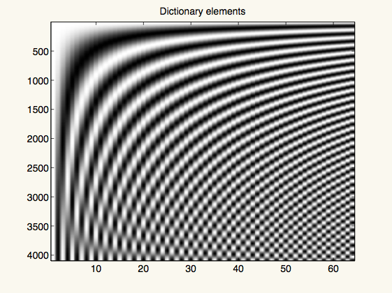
D = zeros(n,m);
for i = 1:m
   D(:,i) = cos((i - 1) * pi * (1:n) / n);
end

% plot a view of the whole dictionary
figure(1)
imagesc(D)
title('Dictionary elements')
colormap(gray(256))

% plot first dictionary elements (cosine functions)
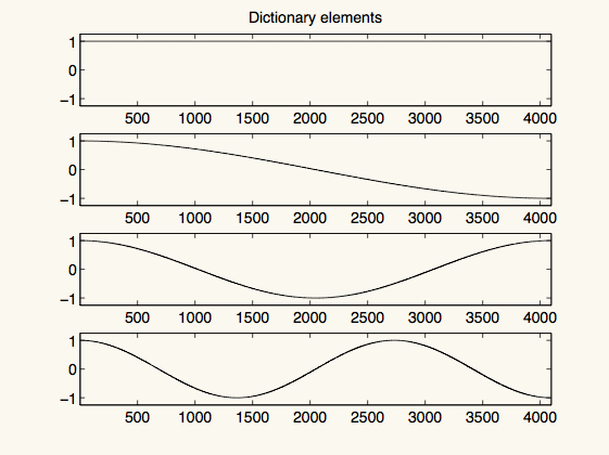
figure(2)
subplot(4,1,1)
plot(D(:,1),'k-')
axis(axf)
title('Dictionary elements')
subplot(4,1,2)
plot(D(:,2),'k-')
axis(axf)
subplot(4,1,3)
plot(D(:,3),'k-')
axis(axf)
subplot(4,1,4)
plot(D(:,4),'k-')
axis(axf)

% constants for sampling the original signal
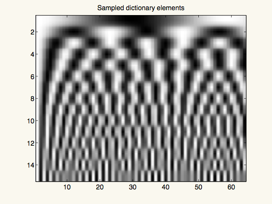
rng(42) % reproduce the exact same experiment
tau = 0.6180339887498948; % golden section conjugate

% try regular, pseudo-random and quasi-random uniform sampling
%k = floor(((0:s-1)' / s) * n + 1); % regular (generates aliasing)
%k = sort(randperm(n,s)'); % pseudo-random
k = sort(floor(((1:s)' * tau - floor((1:s)' * tau)) * n + 1)); % quasi-random

% system matrix: retain only rows corresponding to the s samples
A = zeros(s,m);
for i = 1:s
   A(i,:) = D(k(i),:);
end

% plot a view of the whole system matrix
figure(3)
imagesc(A)
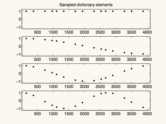
title('Sampled dictionary elements')
colormap(gray(256))

% plot first system matrix columns (sampled cosine functions)
figure(4)
subplot(4,1,1)
plot(k, A(:,1),'k.')
axis(axf)
title('Sampled dictionary elements')
subplot(4,1,2)
plot(k, A(:,2),'k.')
axis(axf)
subplot(4,1,3)
plot(k, A(:,3),'k.')
axis(axf)
subplot(4,1,4)
plot(k, A(:,4),'k.')
axis(axf)

% choose a sparse vector of coefficients
x = zeros(m,1);
x(1) = 0.1; % DC coefficient
x(2) = 0.75;
x(7) = 0.25;
x(23) = 0.1;

% the signal is sparse if few coefficients are significant
sparsity = sum(x > 0) % number of non-zero coefficients in the original signal

% synthesize the original signal
f = sum(D*x,2);

% add Gaussian noise to generate imperfect samples
fn = f + randn(n,1) * 0.05;

% sample the noisy signal
b = fn(k);

% plot the original signal and the noisy samples
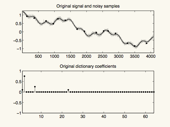
figure(5)
subplot(2,1,1)
plot(fn,'k-','color',[1,1,1]*0.75)
hold on
plot(sum(D*x,2),'k-')
plot(k,b,'k.')
hold off
axis(axf)
title('Original signal and noisy samples')
subplot(2,1,2)
stem(x,'k.')
axis(axd)
title('Original dictionary coefficients')

% Iterative Reweighted Least Square for Sparse Recovery (IRLS)
x = ones(m,1); % uniform weight for first iteration
for l=1:1000 % number of iterations
    x = A' * ((A * ((abs(x) * ones(1,s)).*A')) \ b) .* abs(x);
end

% plot the minimum l1-norm reconstruction
figure(6)
subplot(2,1,1)
stem(x,'k.')
axis(axd)
title('Recovered coefficients')
subplot(2,1,2)
plot(f,'k-','color',[1,1,1] * 0.75)
hold on
plot(sum(D*x,2),'k-')
plot(k,b,'k.')
hold off
axis(axf)
title('Reconstructed signal')

% sort coefficients in descending order
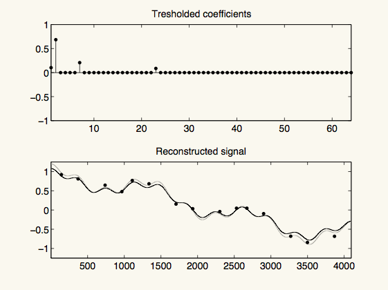
[sortedValues,sortIndex] = sort(abs(x),'descend');

% keep the most significant coefficients (thresholding)
x(sortIndex((sparsity + 1):m)) = 0;

% plot the denoised reconstruction
figure(7)
subplot(2,1,1)
stem(x,'k.')
axis(axd)
title('Tresholded coefficients')
subplot(2,1,2)
plot(f,'k-','color',[1,1,1] * 0.75)
hold on
plot(sum(D*x,2),'k-')
plot(k,b,'k.')
hold off
axis(axf)
title('Reconstructed signal')